Principal Component Analysis
Test post using RStudio.
- New file -> R Markdown -> output as HTML
- Write post as usual and save as .Rmd file
- Knit as HTML and check output
- Once happy with output, change the output to:
output:
  md_document:
    variant: markdown_github
- Then knit and move files to your Jekyll directory accordingly
- If you have images, create a directory in the format
post_category/year/month/date. For this post, the directory isstatistics/2017/01/22
Data set
Using the iris data set.
head(iris)
##   Sepal.Length Sepal.Width Petal.Length Petal.Width Species
## 1          5.1         3.5          1.4         0.2  setosa
## 2          4.9         3.0          1.4         0.2  setosa
## 3          4.7         3.2          1.3         0.2  setosa
## 4          4.6         3.1          1.5         0.2  setosa
## 5          5.0         3.6          1.4         0.2  setosa
## 6          5.4         3.9          1.7         0.4  setosa
Principal Component Analysis
Using prcomp
my_pca <- prcomp(iris[,-5])
my_pca
## Standard deviations:
## [1] 2.0562689 0.4926162 0.2796596 0.1543862
##
## Rotation:
##                      PC1         PC2         PC3        PC4
## Sepal.Length  0.36138659 -0.65658877  0.58202985  0.3154872
## Sepal.Width  -0.08452251 -0.73016143 -0.59791083 -0.3197231
## Petal.Length  0.85667061  0.17337266 -0.07623608 -0.4798390
## Petal.Width   0.35828920  0.07548102 -0.54583143  0.7536574
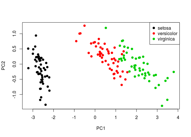
Including Plots
Plot first and second principal components.
plot(my_pca$x[,1], my_pca$x[,2], col = iris$Species, xlab = "PC1", ylab = "PC2", pch=19)
legend('topright', legend = levels(iris$Species), col = 1:3, pch = rep(19,3))
blog comments powered by Disqus